
Introduction
The vote to leave the EU against remaining was made by 52% of all voters (it was a total vote, not number of Wards). These ward-level voting results are published on www.bbc.co.uk/news/uk-politics-38762034. It should be noted that it represents a good proportion of wards, but not all of them. This data is combined with demographic values from www.lgbce.org.uk.
To see which variables are helpful for classification of voting leave or remain, we ran analysis through logistic regression. We could have used linear regression to try and predict the leave/remain numerical vote outcome of any ward or set of demographics whhich could still be used to see if over 50% therefore indicating a binary decision to leave or remain.
Executive Summary
We were successful in creating a model which could predict 94.8% of the vote to leave, based on the basic profile and demographics or any ward, which is an excellent result.
- Deeper analysis of demographic groupings revealed further likelihoods, including:
- The bigger the voting turnout, the more likely remain won the vote. The higher the population density, the more likely remain too.
- As age increased, the more likely a leave vote was passed.
- Level 4 and above qualifications (ie from Diplomas and upwards) were less likely to vote leave. Apprentices were more than twice as likely to vote leave (together, to a lesser extent, those with Level 2).
- Mixed.White.Black.Caribbean were more likely to vote leave, whereas even more likely were Mixed.White.Asian, Other.Mixed and to a lesser extent Chinese to vote remain. White.Gypsy.or.Irish.Traveller were substantially more likely to vote leave, but not enough data confidence to confirm the opposite vote from White.Irish. Arabs were more likely to vote leave, together with Other.Ethnicity. Not as significant (but greater in number) is that White.British were more likely to vote leave.
- PT.Self.Employed were likely to vote remain, followed by Students.Economically.Inactive and FT.Employed. Whereas FT.Self.Employed were more likely to vote leave. Economically.Inactive.Other and Economically.Inactive.Disabled were also likely to vote leave.
- Shared Ownership voters are likely to remain, which also applied to Private Renters. Owners with Mortgages and Social Renters (eg council tenants) were both more likely to vote leave.
- Those in Fair Health were the only grouping likely to vote leave – all other more extreme groupings were more likely to remain, significantly so for both Very Bad Health and Very Good Health.
- Voters with ‘no religion’ were likely to vote remain, followed by Hindu’s, Muslims and Buddhists. All other faiths were non significant at voting either way.
Data Description
For each of 1,030 Ward level counts, there are 63 demographic variables.
Data Preparation
Records are clean, we just need to compute any ratios and remove any incomplete data.
brexitvote <- read.csv('Data\\BrexitVotingAndWardDemographicData.csv')
brexitvote$WardCode <- as.character(brexitvote$WardCode) # WardCode is unique, careful as Ward Name is not
brexitvote$WardName <- as.character(brexitvote$WardName)
brexitvote$CountingArea <- as.character(brexitvote$CountingArea)

rownames(brexitvote) <- brexitvote$WardCode

brexitvote <- droplevels( brexitvote[-which(brexitvote$Outcome == "Draw"), ] )

#brexitvote$Outcome <- as.factor(ifelse(test=brexitvote$Outcome == 'Leave', yes=1, no=0))
brexitvote$Outcome <- as.factor(ifelse(test=brexitvote$Outcome == 'Leave', yes=TRUE, no=FALSE))
#brexitvote <- subset(brexitvote, select = -c(Outcome) ) # Remove if not required

brexitvote$PercLeave <- brexitvote$Leave / (brexitvote$Leave + brexitvote$Remain) # Hold back as collinear to Outcome
brexitvote$PercFemales <- brexitvote$Females / (brexitvote$Females + brexitvote$Males) # Causes issues
brexitvote$Turnout <- (brexitvote$Remain + brexitvote$Leave) / brexitvote$Population.over.16

brexitvote <- subset(brexitvote, select = -c(Remain,Leave) ) # remove Remain and Leave counts (collinear)
brexitvote <- subset(brexitvote, select = -c(Males,Females) ) # replaced by Perc
brexitvote <- subset(brexitvote, select = -c(WardCode,WardName,CountingArea) ) # remove Wards
brexitvote <- subset(brexitvote, select = -c(Mean.Age) ) # Median usually slightly higher but close and only need one.

brexitvote <- na.omit(brexitvote) # Remove NA obs
# str(brexitvote) View(brexitvote)

## Quick analysis only
# model <- glm(Outcome ~ ., data=brexitvote, family=binomial(link='logit'), maxit = 50)
# summary(model)
Data Verification
A quick look at the structure of records.
head(brexitvote)
## Outcome Population Population.over.16 Population.Density ## E05000106 FALSE 15098 12196 31.01 ## E05000107 TRUE 9951 8065 12.01 ## E05000108 TRUE 15113 11978 18.16 ## E05000109 FALSE 16826 13570 45.26 ## E05000110 TRUE 14507 11708 11.55 ## E05000111 FALSE 14831 12164 14.19 ## Number.of.Households Median.Age No.qualification.Percent ## E05000106 5967 42 14.46 ## E05000107 3910 42 18.34 ## E05000108 6209 40 20.46 ## E05000109 7414 37 13.12 ## E05000110 5830 43 16.43 ## E05000111 6084 43 15.78 ## Level.1.qualification.Percent Level.2.qualification.Percent ## E05000106 10.75 15.17 ## E05000107 17.73 18.88 ## E05000108 14.88 16.89 ## E05000109 11.47 14.91 ## E05000110 13.55 17.14 ## E05000111 11.77 15.69 ## Level.3.qualification.Percent ## E05000106 11.54 ## E05000107 13.66 ## E05000108 11.20 ## E05000109 11.95 ## E05000110 12.54 ## E05000111 10.84 ## Level.4.or.above.qualification.Percent ## E05000106 40.73 ## E05000107 22.95 ## E05000108 28.26 ## E05000109 40.99 ## E05000110 33.17 ## E05000111 38.03 ## Apprenticeship.qualifications.Percent ## E05000106 1.878 ## E05000107 4.489 ## E05000108 3.456 ## E05000109 1.820 ## E05000110 3.135 ## E05000111 2.770 ## Other.qualifications.Percent White.British White.Irish ## E05000106 5.469 77.92 1.5565 ## E05000107 3.943 93.25 0.5929 ## E05000108 4.859 81.18 1.3829 ## E05000109 5.741 71.07 1.7235 ## E05000110 4.031 86.59 0.9306 ## E05000111 5.122 81.94 1.1395 ## White.Gypsy.or.Irish.Traveller Other.White ## E05000106 0.03312 5.994 ## E05000107 0.02010 2.010 ## E05000108 0.11910 4.533 ## E05000109 0.01783 8.659 ## E05000110 0.01379 2.737 ## E05000111 0.03371 4.909 ## Mixed.White.Black.Caribbean Mixed.White.Black.African ## E05000106 0.6557 0.2583 ## E05000107 0.7537 0.1507 ## E05000108 1.1910 0.4632 ## E05000109 1.2481 0.6478 ## E05000110 0.4963 0.1999 ## E05000111 0.6877 0.2158 ## Mixed.White.Asian Other.Mixed Indian Pakistani Bangladeshi ## E05000106 1.1657 0.7087 3.8879 0.4305 0.3577 ## E05000107 0.2512 0.3115 0.4623 0.1306 0.1708 ## E05000108 0.8933 0.8470 1.5682 0.2713 0.3970 ## E05000109 1.3075 1.2302 3.2212 0.3804 0.3506 ## E05000110 0.7376 0.4274 2.6608 0.2137 0.1723 ## E05000111 0.8900 0.6136 2.3936 0.6406 0.9440 ## Chinese Other.Asian African Caribbean Other.Black Arabs ## E05000106 1.2386 1.881 1.676 0.8743 0.23844 0.41727 ## E05000107 0.1809 0.402 0.402 0.4522 0.01005 0.07034 ## E05000108 0.6286 1.727 2.342 1.2043 0.52935 0.31761 ## E05000109 1.1114 2.354 2.764 1.8127 0.61809 0.58838 ## E05000110 1.1098 1.255 1.358 0.3102 0.15854 0.24126 ## E05000111 1.2676 1.119 1.301 0.6743 0.26971 0.19554 ## Other.Ethnicity FT.Employed PT.Employed FT.Self.Employed ## E05000106 0.7087 35.40 12.08 9.405 ## E05000107 0.3819 38.21 15.42 8.952 ## E05000108 0.4102 34.03 13.80 8.432 ## E05000109 0.8915 43.52 11.64 8.335 ## E05000110 0.3860 36.91 14.75 7.192 ## E05000111 0.7687 34.88 11.21 8.574 ## PT.Self.Employed Students.Economically.Inactive Unemployed ## E05000106 3.559 4.444 2.763 ## E05000107 3.918 3.497 3.348 ## E05000108 3.640 4.425 4.233 ## E05000109 3.626 3.810 3.898 ## E05000110 3.459 3.502 2.776 ## E05000111 4.061 4.546 2.729 ## Retired Economically.Inactive.Looking.after.home ## E05000106 24.17 4.583 ## E05000107 20.88 3.187 ## E05000108 21.69 4.775 ## E05000109 17.79 3.825 ## E05000110 24.28 4.168 ## E05000111 26.33 4.448 ## Economically.Inactive.Disabled Economically.Inactive.Other ## E05000106 2.140 1.459 ## E05000107 1.426 1.153 ## E05000108 2.939 2.037 ## E05000109 1.828 1.732 ## E05000110 1.572 1.384 ## E05000111 1.578 1.644 ## Home.Owned.Outright Home.Owned.On.Loan Shared.Ownership ## E05000106 38.90 41.33 0.4357 ## E05000107 39.05 48.87 0.8696 ## E05000108 33.53 39.64 0.7409 ## E05000109 27.50 37.77 0.9576 ## E05000110 42.88 44.12 0.5660 ## E05000111 40.70 39.23 0.2301 ## Social.Rent Private.Rent Living.Rent.Free Very.bad.health ## E05000106 6.988 11.413 0.9385 1.0134 ## E05000107 4.604 5.729 0.8696 0.6030 ## E05000108 15.703 9.454 0.9341 0.9661 ## E05000109 10.022 22.741 1.0116 0.6538 ## E05000110 4.631 7.118 0.6861 0.6480 ## E05000111 7.117 11.407 1.3149 1.0316 ## Bad.health Fair.Health Good.health Very.Good.Health Christian ## E05000106 2.981 10.836 32.36 52.81 60.90 ## E05000107 2.834 11.014 35.01 50.54 63.48 ## E05000108 3.408 11.725 33.67 50.23 61.19 ## E05000109 2.716 9.979 33.48 53.17 56.71 ## E05000110 2.495 10.843 34.18 51.84 64.22 ## E05000111 2.974 11.476 32.97 51.55 62.48 ## Buddhist Hindu Sikh Muslim Jewish Other.religion No.religion ## E05000106 0.6292 3.2322 0.3577 2.5434 0.4636 0.4173 22.93 ## E05000107 0.2211 0.3517 0.2110 0.5929 0.1809 0.3015 27.56 ## E05000108 0.5029 1.5153 0.2514 2.2365 0.2117 0.2779 26.63 ## E05000109 0.8439 2.3178 0.3506 3.0073 0.4398 0.4101 27.72 ## E05000110 0.4550 1.8750 0.3653 1.1718 0.3240 0.4067 23.54 ## E05000111 0.4113 1.5441 0.4383 2.9196 0.3911 0.3169 23.81 ## Religion.not.stated PercLeave PercFemales Turnout ## E05000106 8.531 0.4426 0.5311 0.7062 ## E05000107 7.105 0.6470 0.5166 0.7934 ## E05000108 7.186 0.5278 0.5307 0.7065 ## E05000109 8.196 0.4266 0.5163 0.6743 ## E05000110 7.645 0.5408 0.5175 0.6368 ## E05000111 7.687 0.4711 0.5293 0.8283
By summarising the values we can also check for outliers – of which there are none.
summary(brexitvote) # View(brexitvote)
## Outcome Population Population.over.16 Population.Density ## FALSE:404 Min. : 1924 Min. : 1627 Min. : 0.34 ## TRUE :625 1st Qu.: 8034 1st Qu.: 6512 1st Qu.: 16.44 ## Median :11653 Median : 9446 Median : 32.84 ## Mean :11003 Mean : 8854 Mean : 40.21 ## 3rd Qu.:13795 3rd Qu.:11106 3rd Qu.: 51.25 ## Max. :23485 Max. :19382 Max. :194.27 ## Number.of.Households Median.Age No.qualification.Percent ## Min. : 776 Min. :20.0 Min. : 1.69 ## 1st Qu.:3374 1st Qu.:34.0 1st Qu.:16.89 ## Median :4866 Median :38.0 Median :22.02 ## Mean :4532 Mean :38.1 Mean :22.79 ## 3rd Qu.:5673 3rd Qu.:42.0 3rd Qu.:28.44 ## Max. :8609 Max. :55.0 Max. :45.83 ## Level.1.qualification.Percent Level.2.qualification.Percent ## Min. : 1.47 Min. : 4.59 ## 1st Qu.:11.41 1st Qu.:13.49 ## Median :13.75 Median :15.70 ## Mean :13.27 Mean :14.93 ## 3rd Qu.:15.61 3rd Qu.:17.01 ## Max. :20.29 Max. :22.53 ## Level.3.qualification.Percent Level.4.or.above.qualification.Percent ## Min. : 6.93 Min. : 6.77 ## 1st Qu.:10.27 1st Qu.:18.00 ## Median :11.52 Median :25.06 ## Mean :11.95 Mean :27.45 ## 3rd Qu.:12.57 3rd Qu.:34.94 ## Max. :49.32 Max. :68.28 ## Apprenticeship.qualifications.Percent Other.qualifications.Percent ## Min. : 0.183 Min. : 2.46 ## 1st Qu.: 2.021 1st Qu.: 3.98 ## Median : 3.429 Median : 4.86 ## Mean : 3.421 Mean : 6.19 ## 3rd Qu.: 4.533 3rd Qu.: 7.29 ## Max. :11.846 Max. :21.93 ## White.British White.Irish White.Gypsy.or.Irish.Traveller ## Min. : 3.51 Min. :0.036 Min. :0.0000 ## 1st Qu.:60.18 1st Qu.:0.465 1st Qu.:0.0201 ## Median :85.33 Median :0.830 Median :0.0539 ## Mean :74.83 Mean :1.150 Mean :0.0942 ## 3rd Qu.:93.83 3rd Qu.:1.464 3rd Qu.:0.1123 ## Max. :98.38 Max. :5.763 Max. :1.9083 ## Other.White Mixed.White.Black.Caribbean Mixed.White.Black.African ## Min. : 0.244 Min. :0.000 Min. :0.000 ## 1st Qu.: 1.258 1st Qu.:0.358 1st Qu.:0.105 ## Median : 2.769 Median :0.645 Median :0.228 ## Mean : 5.482 Mean :0.971 Mean :0.363 ## 3rd Qu.: 7.000 3rd Qu.:1.300 3rd Qu.:0.509 ## Max. :30.047 Max. :6.347 Max. :1.962 ## Mixed.White.Asian Other.Mixed Indian Pakistani ## Min. :0.0454 Min. :0.000 Min. : 0.00 Min. : 0.00 ## 1st Qu.:0.3321 1st Qu.:0.215 1st Qu.: 0.45 1st Qu.: 0.19 ## Median :0.6280 Median :0.394 Median : 1.32 Median : 0.53 ## Mean :0.7537 Mean :0.665 Mean : 3.39 Mean : 2.76 ## 3rd Qu.:1.1097 3rd Qu.:0.986 3rd Qu.: 3.11 3rd Qu.: 1.83 ## Max. :2.9358 Max. :2.931 Max. :54.67 Max. :72.30 ## Bangladeshi Chinese Other.Asian African ## Min. : 0.00 Min. :0.000 Min. : 0.000 Min. : 0.00 ## 1st Qu.: 0.08 1st Qu.:0.251 1st Qu.: 0.333 1st Qu.: 0.22 ## Median : 0.27 Median :0.486 Median : 0.910 Median : 0.75 ## Mean : 0.91 Mean :0.771 Mean : 2.025 Mean : 2.30 ## 3rd Qu.: 0.80 3rd Qu.:0.932 3rd Qu.: 2.488 3rd Qu.: 2.54 ## Max. :60.34 Max. :8.639 Max. :22.108 Max. :35.58 ## Caribbean Other.Black Arabs Other.Ethnicity ## Min. : 0.000 Min. :0.000 Min. :0.000 Min. :0.000 ## 1st Qu.: 0.130 1st Qu.:0.049 1st Qu.:0.056 1st Qu.:0.128 ## Median : 0.337 Median :0.149 Median :0.160 Median :0.343 ## Mean : 1.574 Mean :0.699 Mean :0.435 Mean :0.817 ## 3rd Qu.: 1.781 3rd Qu.:0.719 3rd Qu.:0.545 3rd Qu.:1.071 ## Max. :20.999 Max. :7.734 Max. :8.553 Max. :7.245 ## FT.Employed PT.Employed FT.Self.Employed PT.Self.Employed ## Min. :11.6 Min. : 6.27 Min. : 1.50 Min. :0.781 ## 1st Qu.:32.9 1st Qu.:13.28 1st Qu.: 4.65 1st Qu.:1.868 ## Median :35.8 Median :14.29 Median : 5.85 Median :2.499 ## Mean :35.9 Mean :14.08 Mean : 6.11 Mean :2.715 ## 3rd Qu.:38.9 3rd Qu.:15.22 3rd Qu.: 7.49 3rd Qu.:3.403 ## Max. :59.1 Max. :22.12 Max. :13.12 Max. :7.156 ## Students.Economically.Inactive Unemployed Retired ## Min. : 1.73 Min. : 1.20 Min. : 5.17 ## 1st Qu.: 3.36 1st Qu.: 3.48 1st Qu.:14.87 ## Median : 4.11 Median : 4.88 Median :20.31 ## Mean : 5.50 Mean : 5.17 Mean :19.81 ## 3rd Qu.: 5.95 3rd Qu.: 6.50 3rd Qu.:24.37 ## Max. :56.88 Max. :13.25 Max. :42.77 ## Economically.Inactive.Looking.after.home Economically.Inactive.Disabled ## Min. : 0.92 Min. : 0.422 ## 1st Qu.: 3.09 1st Qu.: 2.503 ## Median : 3.88 Median : 3.740 ## Mean : 4.24 Mean : 4.125 ## 3rd Qu.: 4.97 3rd Qu.: 5.299 ## Max. :15.30 Max. :12.646 ## Economically.Inactive.Other Home.Owned.Outright Home.Owned.On.Loan ## Min. : 0.532 Min. : 4.76 Min. : 7.55 ## 1st Qu.: 1.470 1st Qu.:20.79 1st Qu.:27.77 ## Median : 2.009 Median :28.21 Median :33.79 ## Mean : 2.363 Mean :28.80 Mean :32.87 ## 3rd Qu.: 2.900 3rd Qu.:36.47 3rd Qu.:38.73 ## Max. :13.661 Max. :63.49 Max. :62.78 ## Shared.Ownership Social.Rent Private.Rent Living.Rent.Free ## Min. :0.000 Min. : 0.48 Min. : 3.89 Min. :0.271 ## 1st Qu.:0.272 1st Qu.: 9.10 1st Qu.: 9.75 1st Qu.:0.883 ## Median :0.509 Median :16.43 Median :13.78 Median :1.142 ## Mean :0.771 Mean :19.36 Mean :16.96 Mean :1.238 ## 3rd Qu.:1.049 3rd Qu.:27.32 3rd Qu.:22.80 3rd Qu.:1.468 ## Max. :7.388 Max. :67.03 Max. :60.68 Max. :5.918 ## Very.bad.health Bad.health Fair.Health Good.health ## Min. :0.185 Min. :0.973 Min. : 5.23 Min. :26.6 ## 1st Qu.:0.954 1st Qu.:3.317 1st Qu.:11.55 1st Qu.:32.9 ## Median :1.240 Median :4.233 Median :13.18 Median :34.3 ## Mean :1.300 Mean :4.422 Mean :13.14 Mean :34.2 ## 3rd Qu.:1.600 3rd Qu.:5.379 3rd Qu.:14.89 3rd Qu.:35.6 ## Max. :3.443 Max. :9.361 Max. :19.36 Max. :40.0 ## Very.Good.Health Christian Buddhist Hindu ## Min. :34.9 Min. : 7.66 Min. :0.000 Min. : 0.00 ## 1st Qu.:43.6 1st Qu.:50.93 1st Qu.:0.188 1st Qu.: 0.21 ## Median :46.3 Median :59.97 Median :0.320 Median : 0.66 ## Mean :47.0 Mean :57.88 Mean :0.507 Mean : 2.02 ## 3rd Qu.:49.7 3rd Qu.:67.48 3rd Qu.:0.692 3rd Qu.: 1.77 ## Max. :65.4 Max. :84.36 Max. :3.573 Max. :45.34 ## Sikh Muslim Jewish Other.religion ## Min. : 0.00 Min. : 0.00 Min. : 0.00 Min. :0.026 ## 1st Qu.: 0.08 1st Qu.: 0.66 1st Qu.: 0.03 1st Qu.:0.255 ## Median : 0.22 Median : 2.04 Median : 0.11 Median :0.360 ## Mean : 1.05 Mean : 6.34 Mean : 0.53 Mean :0.465 ## 3rd Qu.: 0.60 3rd Qu.: 7.57 3rd Qu.: 0.30 3rd Qu.:0.516 ## Max. :39.42 Max. :85.32 Max. :40.96 Max. :8.180 ## No.religion Religion.not.stated PercLeave PercFemales ## Min. : 1.48 Min. : 4.15 Min. :0.122 Min. :0.414 ## 1st Qu.:19.34 1st Qu.: 6.13 1st Qu.:0.432 1st Qu.:0.507 ## Median :23.54 Median : 6.75 Median :0.552 Median :0.515 ## Mean :23.97 Mean : 7.25 Mean :0.525 Mean :0.513 ## 3rd Qu.:28.56 3rd Qu.: 7.62 3rd Qu.:0.641 3rd Qu.:0.523 ## Max. :55.70 Max. :25.64 Max. :0.790 Max. :0.565 ## Turnout ## Min. :0.255 ## 1st Qu.:0.551 ## Median :0.627 ## Mean :0.640 ## 3rd Qu.:0.706 ## Max. :1.657
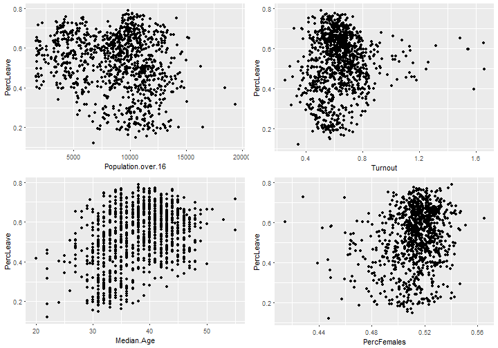
Data Distribution
Let’s check the key variable frequency distributions.
We can see that although all these variables are right-skewed (tend towards the bigger values) they are all uni-modal and have no large outliers so can be considered as normal.
If they were standardised into z-scores, they would be centralised along their average means and even more balanced.
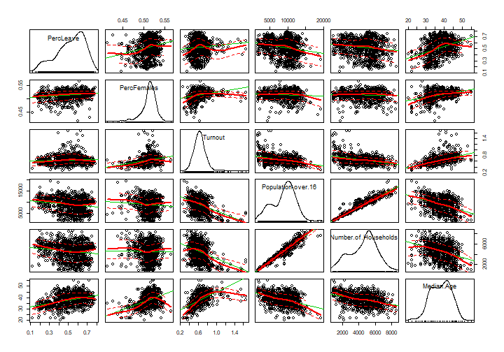
Correlations and Preliminaries
Let’s check correlation (without the splits of Education, Race, Employment, Home Ownership, Health or Religion). ## PercLeave PercFemales Turnout Population.over.16 ## PercLeave 1.00000 0.20176 0.07898 -0.19801 ## PercFemales 0.20176 1.00000 0.25246 -0.07612 ## Turnout 0.07898 0.25246 1.00000 -0.38591 ## Population.over.16 -0.19801 -0.07612 -0.38591 1.00000 ## Number.of.Households -0.14883 -0.01226 -0.34877 0.96715 ## Median.Age 0.38333 0.39482 0.52154 -0.40874 ## Number.of.Households Median.Age ## PercLeave -0.14883 0.3833 ## PercFemales -0.01226 0.3948 ## Turnout -0.34877 0.5215 ## Population.over.16 0.96715 -0.4087 ## Number.of.Households 1.00000 -0.3384 ## Median.Age -0.33845 1.0000
We can see the relationships are fairly centralised regarding the Percentage Leave vote which the outcome is based on, so no obvious influences.
We can see the confidence intervals tighten to improve in the mid ranges of the variables, which is expected. As we have a good number of cases, we needn’t worry about the widening intervals at outer ranges.
Data Assumptions
Unlike linear regression, logistic regression is not so sensitive to its data being normally distributed.
We can assume that the observations are all independant, especially becasue they are counts per ward and not individual personal cases.
The model is fitted using binomial logistical regression with a logit link function. We need to remove our percentage of leavers becasue it’s collinear with the final Outcome (Leave or Remain). Then we can check residuals – as mentioned, it is not a prerequisite to have normal distribution of error differences.
These residual plots show the familiar patterns of logistic regression (due to the binary nature of outcome response) so are acceptable.
Logistic Regression
Now we can inspect the model statistics. Logistic Regression does not have an R-Squared value to indicate cover of true response variability, so is more difficult to verify goodness of fit.
Coefficient estimates (weighting of influence) are based on the outcome response of voting leave (the majority). They’re measured in log odds (aka logit) and are not as simple to interpret as many analysts believe. The baseline is 1 which represents no change, whilst 1.5 would represent “one and a half times more likely”. However, these positive numbers can increase right up the scale.
Note, when we say something is “significantly more likely” we don’t mean that it’s culturally significant or even more likely in comparison to other factors (unless stated specifically) – by “significantly” we mean the observation is significantly unlikely to occur by chance, ie we can be more confident that it is a true statement about the data.
Also, we can only talk about particular groups being “more likely” to vote one way, but this is a geralisation, because ultimately we only have counts by ward, not individual observations. So in such cases we are effectively saying that a ward is more likely to vote one way given a higher proportion of that group, with all other variables held constant.
Population, Age and Turnout
Let’s check the significance and effect of the non-demographic variables.
brexitvote.sub <- subset(brexitvote, select = c(Outcome, Population, Population.over.16, Population.Density,  Number.of.Households, Median.Age, Turnout) )

model <- glm(Outcome ~ ., data=brexitvote.sub, family=binomial(link='logit'), maxit = 50)
summary(model)
## ## Call: ## glm(formula = Outcome ~ ., family = binomial(link = “logit”), ## data = brexitvote.sub, maxit = 50) ## ## Deviance Residuals: ## Min 1Q Median 3Q Max ## -2.409 -0.827 0.572 0.817 2.369 ## ## Coefficients: ## Estimate Std. Error z value Pr(>|z|) ## (Intercept) 0.818470 0.962376 0.85 0.39507 ## Population 0.000571 0.000161 3.55 0.00039 *** ## Population.over.16 -0.001380 0.000251 -5.49 4.0e-08 *** ## Population.Density -0.030397 0.003862 -7.87 3.5e-15 *** ## Number.of.Households 0.001234 0.000216 5.71 1.2e-08 *** ## Median.Age 0.083899 0.022514 3.73 0.00019 *** ## Turnout -3.144057 0.616303 -5.10 3.4e-07 *** ## — ## Signif. codes: 0 ‘***’ 0.001 ‘**’ 0.01 ‘*’ 0.05 ‘.’ 0.1 ‘ ‘ 1 ## ## (Dispersion parameter for binomial family taken to be 1) ## ## Null deviance: 1378.7 on 1028 degrees of freedom ## Residual deviance: 1074.4 on 1022 degrees of freedom ## AIC: 1088 ## ## Number of Fisher Scoring iterations: 5
To help interpret the coefficient Estimate, we can convert it into an Odds Ratio. ## Coefficients Odds.Ratio ## (Intercept) 0.818470 2.2670 ## Median.Age 0.083899 1.0875 ## Number.of.Households 0.001234 1.0012 ## Population 0.000571 1.0006 ## Population.over.16 -0.001380 0.9986 ## Population.Density -0.030397 0.9701 ## Turnout -3.144057 0.0431
All factors are highly significant, with the highest effect from Turnout – the bigger the voting turnout, the more likely remain won the vote. The higher the population density, the more likely remain too. As age increased, the more likely a leave vote was passed.
Turning to the demographics, we’ll keep them split to focus estimations within the groups, otherwise they get watered down.
Education / Qualifications
## ## Call: ## glm(formula = Outcome ~ ., family = binomial(link = “logit”), ## data = brexitvote.sub, maxit = 50) ## ## Deviance Residuals: ## Min 1Q Median 3Q Max ## -3.039 -0.199 0.139 0.366 3.414 ## ## Coefficients: (1 not defined because of singularities) ## Estimate Std. Error z value ## (Intercept) -0.3027 4.8147 -0.06 ## No.qualification.Percent -0.0372 0.0600 -0.62 ## Level.1.qualification.Percent 0.0234 0.1266 0.19 ## Level.2.qualification.Percent 0.3017 0.0971 3.11 ## Level.3.qualification.Percent -0.0437 0.0622 -0.70 ## Level.4.or.above.qualification.Percent -0.2044 0.0611 -3.34 ## Apprenticeship.qualifications.Percent 0.8656 0.1271 6.81 ## Other.qualifications.Percent NA NA NA ## Pr(>|z|) ## (Intercept) 0.94987 ## No.qualification.Percent 0.53556 ## Level.1.qualification.Percent 0.85317 ## Level.2.qualification.Percent 0.00189 ** ## Level.3.qualification.Percent 0.48279 ## Level.4.or.above.qualification.Percent 0.00083 *** ## Apprenticeship.qualifications.Percent 9.6e-12 *** ## Other.qualifications.Percent NA ## — ## Signif. codes: 0 ‘***’ 0.001 ‘**’ 0.01 ‘*’ 0.05 ‘.’ 0.1 ‘ ‘ 1 ## ## (Dispersion parameter for binomial family taken to be 1) ## ## Null deviance: 1378.66 on 1028 degrees of freedom ## Residual deviance: 528.48 on 1022 degrees of freedom ## AIC: 542.5 ## ## Number of Fisher Scoring iterations: 7 ## Coefficients Odds.Ratio ## Apprenticeship.qualifications.Percent 0.8656 2.376 ## Level.2.qualification.Percent 0.3017 1.352 ## Level.1.qualification.Percent 0.0234 1.024 ## No.qualification.Percent -0.0372 0.964 ## Level.3.qualification.Percent -0.0437 0.957 ## Level.4.or.above.qualification.Percent -0.2044 0.815 ## (Intercept) -0.3027 0.739 ## Other.qualifications.Percent NA NA
Note the NAs (and “1 not defined because of singularities”) result from each grouping at ward level adding up to 100%, so each last remaining group category is effectively collinear. We can remove them but they have no effect on the model coefficients or summary statistics and keep the groupings and category names clearer.
From this result, it appears highly significant that Level 4 and above qualifications (ie from Diplomas and upwards) were less likely to vote leave. Apprentices were more than twice as likely to vote leave (together, to a lesser extent, those with Level 2).
We should be careful of which group is the baseline reference group, because if, like in this case, the last group is chosen, it is likely to be the smallest group, which then inflates the influence of the other groups. Generally, the largest group should be chosen for the baseline, however this is often one of the contentious groups we want visibility of. We will use a mid-range group here – Level 2 qualifications. ## ## Call: ## glm(formula = Outcome ~ ., family = binomial(link = “logit”), ## data = brexitvote.sub, maxit = 50) ## ## Deviance Residuals: ## Min 1Q Median 3Q Max ## -3.039 -0.199 0.139 0.366 3.414 ## ## Coefficients: ## Estimate Std. Error z value ## (Intercept) 29.8686 10.3124 2.90 ## No.qualification.Percent -0.3389 0.1068 -3.17 ## Level.1.qualification.Percent -0.2783 0.1909 -1.46 ## Level.3.qualification.Percent -0.3454 0.1178 -2.93 ## Level.4.or.above.qualification.Percent -0.5061 0.1167 -4.34 ## Apprenticeship.qualifications.Percent 0.5639 0.1991 2.83 ## Other.qualifications.Percent -0.3017 0.0971 -3.11 ## Pr(>|z|) ## (Intercept) 0.0038 ** ## No.qualification.Percent 0.0015 ** ## Level.1.qualification.Percent 0.1449 ## Level.3.qualification.Percent 0.0034 ** ## Level.4.or.above.qualification.Percent 1.5e-05 *** ## Apprenticeship.qualifications.Percent 0.0046 ** ## Other.qualifications.Percent 0.0019 ** ## — ## Signif. codes: 0 ‘***’ 0.001 ‘**’ 0.01 ‘*’ 0.05 ‘.’ 0.1 ‘ ‘ 1 ## ## (Dispersion parameter for binomial family taken to be 1) ## ## Null deviance: 1378.66 on 1028 degrees of freedom ## Residual deviance: 528.48 on 1022 degrees of freedom ## AIC: 542.5 ## ## Number of Fisher Scoring iterations: 7 ## Coefficients Odds.Ratio ## (Intercept) 29.869 9.37e+12 ## Apprenticeship.qualifications.Percent 0.564 1.76e+00 ## Level.1.qualification.Percent -0.278 7.57e-01 ## Other.qualifications.Percent -0.302 7.40e-01 ## No.qualification.Percent -0.339 7.13e-01 ## Level.3.qualification.Percent -0.345 7.08e-01 ## Level.4.or.above.qualification.Percent -0.506 6.03e-01
We can see it remains highly significant that Level 4 or above is even more likely to vote remain. This regrouping has allowed the “No Qualifications” group to seen as significant and in fact all groups apart from Apprentices contribute to the vote to remain.
Race / Ethnicity
For race / ethnicity, we’ll choose the non-extreme “Other White” for baseline – it’s still minority but the next largest grouping. ## ## Call: ## glm(formula = Outcome ~ ., family = binomial(link = “logit”), ## data = brexitvote.sub, maxit = 50) ## ## Deviance Residuals: ## Min 1Q Median 3Q Max ## -2.705 -0.288 0.334 0.530 2.778 ## ## Coefficients: ## Estimate Std. Error z value Pr(>|z|) ## (Intercept) -5.6727 4.8769 -1.16 0.2448 ## White.British 0.0872 0.0486 1.80 0.0724 . ## White.Irish -0.2932 0.1879 -1.56 0.1187 ## White.Gypsy.or.Irish.Traveller 3.2495 1.1305 2.87 0.0040 ** ## Mixed.White.Black.Caribbean 1.5590 0.2246 6.94 3.9e-12 *** ## Mixed.White.Black.African 0.2910 0.7241 0.40 0.6877 ## Mixed.White.Asian -1.9767 0.4215 -4.69 2.7e-06 *** ## Other.Mixed -1.9453 0.6856 -2.84 0.0045 ** ## Indian 0.0479 0.0510 0.94 0.3482 ## Pakistani 0.0420 0.0504 0.83 0.4045 ## Bangladeshi 0.0454 0.0583 0.78 0.4361 ## Chinese -0.8485 0.2187 -3.88 0.0001 *** ## Other.Asian 0.2122 0.0767 2.77 0.0057 ** ## African 0.1388 0.0859 1.62 0.1062 ## Caribbean -0.1238 0.1552 -0.80 0.4251 ## Other.Black -0.1788 0.3886 -0.46 0.6453 ## Arabs 0.4271 0.2142 1.99 0.0461 * ## Other.Ethnicity 0.5035 0.2177 2.31 0.0207 * ## — ## Signif. codes: 0 ‘***’ 0.001 ‘**’ 0.01 ‘*’ 0.05 ‘.’ 0.1 ‘ ‘ 1 ## ## (Dispersion parameter for binomial family taken to be 1) ## ## Null deviance: 1378.66 on 1028 degrees of freedom ## Residual deviance: 727.33 on 1011 degrees of freedom ## AIC: 763.3 ## ## Number of Fisher Scoring iterations: 6
Most significant (data confidence wise) is that Mixed.White.Black.Caribbean is more likely to vote leave, whereas even more likely are Mixed.White.Asian, Other.Mixed and to a lesser extent Chinese to vote remain. However, Other.Asian are more likely to vote leave, so that could combine with the Mixed.White.Asian to even out.
White.Gypsy.or.Irish.Traveller are substantially more likely to vote leave, whilst there’s not enough data confidence to confirm the opposite vote from White.Irish. Not as significant (albeit greater in number) is that White.British are more likely to vote leave.
Arabs are more likely to vote leave, together with Other.Ethnicity.
Employment Status
For Employment status, we use PT.Employed as baseline. ## ## Call: ## glm(formula = Outcome ~ ., family = binomial(link = “logit”), ## data = brexitvote.sub, maxit = 50) ## ## Deviance Residuals: ## Min 1Q Median 3Q Max ## -3.029 -0.337 0.201 0.436 2.703 ## ## Coefficients: ## Estimate Std. Error z value ## (Intercept) 22.8306 6.0512 3.77 ## FT.Employed -0.2982 0.0741 -4.03 ## FT.Self.Employed 0.5717 0.1302 4.39 ## PT.Self.Employed -3.0143 0.2859 -10.54 ## Students.Economically.Inactive -0.5912 0.0996 -5.93 ## Unemployed 0.1328 0.1335 1.00 ## Retired -0.1178 0.0776 -1.52 ## Economically.Inactive.Looking.after.home -0.0415 0.1264 -0.33 ## Economically.Inactive.Disabled -0.2108 0.1071 -1.97 ## Economically.Inactive.Other -0.4121 0.1268 -3.25 ## Pr(>|z|) ## (Intercept) 0.00016 *** ## FT.Employed 5.7e-05 *** ## FT.Self.Employed 1.1e-05 *** ## PT.Self.Employed < 2e-16 *** ## Students.Economically.Inactive 3.0e-09 *** ## Unemployed 0.31963 ## Retired 0.12913 ## Economically.Inactive.Looking.after.home 0.74242 ## Economically.Inactive.Disabled 0.04900 * ## Economically.Inactive.Other 0.00116 ** ## — ## Signif. codes: 0 ‘***’ 0.001 ‘**’ 0.01 ‘*’ 0.05 ‘.’ 0.1 ‘ ‘ 1 ## ## (Dispersion parameter for binomial family taken to be 1) ## ## Null deviance: 1378.66 on 1028 degrees of freedom ## Residual deviance: 648.32 on 1019 degrees of freedom ## AIC: 668.3 ## ## Number of Fisher Scoring iterations: 6
PT.Self.Employed are most likely to vote remain, followed by Students.Economically.Inactive and FT.Employed. Whereas FT.Self.Employed are more likely to vote leave.
Economically.Inactive.Other and Economically.Inactive.Disabled are also likely to vote leave.
Home Ownership
For home ownership, we use Home.Owned.Outright as baseline. ## ## Call: ## glm(formula = Outcome ~ ., family = binomial(link = “logit”), ## data = brexitvote.sub, maxit = 50) ## ## Deviance Residuals: ## Min 1Q Median 3Q Max ## -2.357 -0.865 0.519 0.750 2.367 ## ## Coefficients: ## Estimate Std. Error z value Pr(>|z|) ## (Intercept) -2.0921 1.0252 -2.04 0.04129 * ## Home.Owned.On.Loan 0.0987 0.0200 4.94 7.9e-07 *** ## Shared.Ownership -0.3835 0.1088 -3.53 0.00042 *** ## Social.Rent 0.0683 0.0109 6.29 3.2e-10 *** ## Private.Rent -0.0925 0.0123 -7.54 4.6e-14 *** ## Living.Rent.Free -0.1024 0.1632 -0.63 0.53046 ## — ## Signif. codes: 0 ‘***’ 0.001 ‘**’ 0.01 ‘*’ 0.05 ‘.’ 0.1 ‘ ‘ 1 ## ## (Dispersion parameter for binomial family taken to be 1) ## ## Null deviance: 1378.7 on 1028 degrees of freedom ## Residual deviance: 1055.5 on 1023 degrees of freedom ## AIC: 1068 ## ## Number of Fisher Scoring iterations: 4
Its most highly significant (data wise) that Shared Ownership voters are likely to remain, which also applies to Private Renters. Owners with Mortgages and Social Renters (eg council tenants) are both more likely to vote leave.
Health
Fair Health is used as the baseline here. ## ## Call: ## glm(formula = Outcome ~ ., family = binomial(link = “logit”), ## data = brexitvote.sub, maxit = 50) ## ## Deviance Residuals: ## Min 1Q Median 3Q Max ## -2.973 -0.665 0.331 0.658 3.015 ## ## Coefficients: ## Estimate Std. Error z value Pr(>|z|) ## (Intercept) 79.2927 9.2184 8.60 < 2e-16 *** ## Very.bad.health -3.3145 0.4499 -7.37 1.7e-13 *** ## Bad.health -0.5911 0.2551 -2.32 0.02 * ## Good.health -0.8133 0.1201 -6.77 1.3e-11 *** ## Very.Good.Health -0.9361 0.0915 -10.23 < 2e-16 *** ## — ## Signif. codes: 0 ‘***’ 0.001 ‘**’ 0.01 ‘*’ 0.05 ‘.’ 0.1 ‘ ‘ 1 ## ## (Dispersion parameter for binomial family taken to be 1) ## ## Null deviance: 1378.66 on 1028 degrees of freedom ## Residual deviance: 898.17 on 1024 degrees of freedom ## AIC: 908.2 ## ## Number of Fisher Scoring iterations: 5
It seems that Fair Health is the only grouping likely to vote leave – all other more extreme groupings are more likely to remain, significantly so for both Very Bad Health and Very Good Health.
Religion
No Religion is convenient to use as baseline here. ## ## Call: ## glm(formula = Outcome ~ ., family = binomial(link = “logit”), ## data = brexitvote.sub, maxit = 50) ## ## Deviance Residuals: ## Min 1Q Median 3Q Max ## -2.541 -0.522 0.326 0.599 2.642 ## ## Coefficients: ## Estimate Std. Error z value Pr(>|z|) ## (Intercept) 13.19954 1.77644 7.43 1.1e-13 *** ## Christian -0.02019 0.01705 -1.18 0.23627 ## Buddhist -0.90968 0.27542 -3.30 0.00096 *** ## Hindu -0.12569 0.03031 -4.15 3.4e-05 *** ## Sikh -0.03521 0.02787 -1.26 0.20650 ## Muslim -0.10356 0.01592 -6.50 7.8e-11 *** ## Jewish 0.00568 0.04690 0.12 0.90359 ## Other.religion 0.19361 0.23772 0.81 0.41538 ## Religion.not.stated -1.45531 0.13577 -10.72 < 2e-16 *** ## — ## Signif. codes: 0 ‘***’ 0.001 ‘**’ 0.01 ‘*’ 0.05 ‘.’ 0.1 ‘ ‘ 1 ## ## (Dispersion parameter for binomial family taken to be 1) ## ## Null deviance: 1378.66 on 1028 degrees of freedom ## Residual deviance: 830.46 on 1020 degrees of freedom ## AIC: 848.5 ## ## Number of Fisher Scoring iterations: 6
It seems most highly significant that those with ‘no religion’ were likely to vote remain, followed by Hindu’s, Muslims and Buddhists. All other faiths were non significant.
Validation with Prediction
The most important test of model is whether it can predict at least or preferable better than the original outcome (without first being given that value).
Let’s use all the variables in the model. ## ## Call: ## glm(formula = Outcome ~ ., family = binomial(link = “logit”), ## data = brexitvote.sub, maxit = 50) ## ## Deviance Residuals: ## Min 1Q Median 3Q Max ## -3.074 -0.067 0.031 0.167 3.639 ## ## Coefficients: ## Estimate Std. Error z value ## (Intercept) 57.3783 85.3871 0.67 ## No.qualification.Percent -0.1061 0.2511 -0.42 ## Level.1.qualification.Percent -0.3397 0.3060 -1.11 ## Level.2.qualification.Percent -0.1099 0.2804 -0.39 ## Level.3.qualification.Percent -0.1920 0.2693 -0.71 ## Level.4.or.above.qualification.Percent -0.5023 0.2275 -2.21 ## Apprenticeship.qualifications.Percent 0.2800 0.3489 0.80 ## White.British -0.8016 0.6004 -1.34 ## White.Irish -0.7801 0.6361 -1.23 ## White.Gypsy.or.Irish.Traveller 2.3675 1.8230 1.30 ## Other.White -0.9567 0.6703 -1.43 ## Mixed.White.Black.Caribbean 0.0823 0.6319 0.13 ## Mixed.White.Black.African -2.6029 1.4188 -1.83 ## Mixed.White.Asian -0.9574 0.9540 -1.00 ## Other.Mixed -1.5040 1.2449 -1.21 ## Indian -0.6572 0.5312 -1.24 ## Pakistani -0.7139 0.5278 -1.35 ## Bangladeshi -0.7360 0.5283 -1.39 ## Chinese -1.7095 0.7252 -2.36 ## Other.Asian -0.8673 0.5728 -1.51 ## African -0.9645 0.6059 -1.59 ## Caribbean -1.4340 0.7032 -2.04 ## Other.Black 0.1986 0.9001 0.22 ## Arabs -0.6202 0.7262 -0.85 ## FT.Employed -0.5579 0.4468 -1.25 ## PT.Employed -1.0148 0.4634 -2.19 ## FT.Self.Employed 0.1021 0.4554 0.22 ## PT.Self.Employed -1.6461 0.6474 -2.54 ## Students.Economically.Inactive -0.5197 0.4680 -1.11 ## Unemployed -0.1853 0.5511 -0.34 ## Retired -0.5407 0.4565 -1.18 ## Economically.Inactive.Looking.after.home -0.2740 0.5474 -0.50 ## Economically.Inactive.Disabled -0.9184 0.6046 -1.52 ## Home.Owned.Outright 0.4161 0.3581 1.16 ## Home.Owned.On.Loan 0.4471 0.3568 1.25 ## Shared.Ownership 0.3912 0.4340 0.90 ## Social.Rent 0.4555 0.3619 1.26 ## Private.Rent 0.4407 0.3659 1.20 ## Very.bad.health 0.7751 1.0010 0.77 ## Bad.health -0.6176 0.5334 -1.16 ## Fair.Health -0.1315 0.2583 -0.51 ## Good.health 0.2623 0.1600 1.64 ## Christian 0.6696 0.2983 2.24 ## Buddhist 1.9975 0.6621 3.02 ## Hindu 0.4014 0.3254 1.23 ## Sikh 0.3430 0.3386 1.01 ## Muslim 0.3230 0.3212 1.01 ## Jewish 0.6922 0.3214 2.15 ## Other.religion 0.5931 0.5979 0.99 ## No.religion 0.5558 0.3314 1.68 ## Pr(>|z|) ## (Intercept) 0.5016 ## No.qualification.Percent 0.6727 ## Level.1.qualification.Percent 0.2668 ## Level.2.qualification.Percent 0.6951 ## Level.3.qualification.Percent 0.4760 ## Level.4.or.above.qualification.Percent 0.0272 * ## Apprenticeship.qualifications.Percent 0.4223 ## White.British 0.1819 ## White.Irish 0.2200 ## White.Gypsy.or.Irish.Traveller 0.1940 ## Other.White 0.1535 ## Mixed.White.Black.Caribbean 0.8963 ## Mixed.White.Black.African 0.0666 . ## Mixed.White.Asian 0.3156 ## Other.Mixed 0.2270 ## Indian 0.2160 ## Pakistani 0.1761 ## Bangladeshi 0.1636 ## Chinese 0.0184 * ## Other.Asian 0.1300 ## African 0.1114 ## Caribbean 0.0414 * ## Other.Black 0.8254 ## Arabs 0.3931 ## FT.Employed 0.2119 ## PT.Employed 0.0285 * ## FT.Self.Employed 0.8225 ## PT.Self.Employed 0.0110 * ## Students.Economically.Inactive 0.2668 ## Unemployed 0.7366 ## Retired 0.2363 ## Economically.Inactive.Looking.after.home 0.6167 ## Economically.Inactive.Disabled 0.1288 ## Home.Owned.Outright 0.2452 ## Home.Owned.On.Loan 0.2102 ## Shared.Ownership 0.3674 ## Social.Rent 0.2082 ## Private.Rent 0.2285 ## Very.bad.health 0.4387 ## Bad.health 0.2470 ## Fair.Health 0.6107 ## Good.health 0.1011 ## Christian 0.0248 * ## Buddhist 0.0026 ** ## Hindu 0.2175 ## Sikh 0.3110 ## Muslim 0.3147 ## Jewish 0.0313 * ## Other.religion 0.3212 ## No.religion 0.0935 . ## — ## Signif. codes: 0 ‘***’ 0.001 ‘**’ 0.01 ‘*’ 0.05 ‘.’ 0.1 ‘ ‘ 1 ## ## (Dispersion parameter for binomial family taken to be 1) ## ## Null deviance: 1378.66 on 1028 degrees of freedom ## Residual deviance: 336.58 on 979 degrees of freedom ## AIC: 436.6 ## ## Number of Fisher Scoring iterations: 8
Then use the model to predict the outcome (Leave or Remain vote), and use a Confusion Table to tabulate the results. ## predicted ## truth FALSE TRUE Sum ## FALSE 374 30 404 ## TRUE 32 593 625 ## Sum 406 623 1029
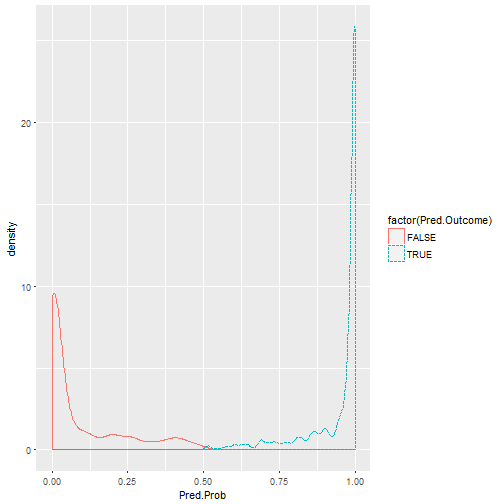
## Sensitivity/Recall (TP) = 0.949 ## Specificity (TN) = 0.926 ## Positive Predictive Value / Precision (All P) = 0.952 ## Negative Predictive Value (All N) = 0.921 ## Overall Accuracy / Hit-rate= 0.94
We have an overall accuracy of 94%, which is very good (especially considering all the factors which make somebody vote either way). Note that this accuracy statistic can be misleading for non-equal category sizes, which most data is, but considering the vote outcome was close at 52% Leave, our accuracy here is pretty impressive.
Training and Validation
Now we’ll split the dataset into training and validation, and only give the model 70% of the dataset to train on, leaving the other 30% for it to predict. ## [1] “Training Confusion Matrix” ## predicted ## truth FALSE TRUE Sum ## FALSE 265 22 287 ## TRUE 24 409 433 ## Sum 289 431 720 ## [1] “Validation Confusion Matrix” ## predicted ## truth FALSE TRUE Sum ## FALSE 109 8 117 ## TRUE 8 184 192 ## Sum 117 192 309 ## [1] “Training Probability”

## Sensitivity/Recall (TP) = 0.945 ## Specificity (TN) = 0.923 ## Positive Predictive Value / Precision (All P) = 0.949 ## Negative Predictive Value (All N) = 0.917 ## Overall Accuracy / Hit-rate= 0.936 ## [1] “Validation Probability”
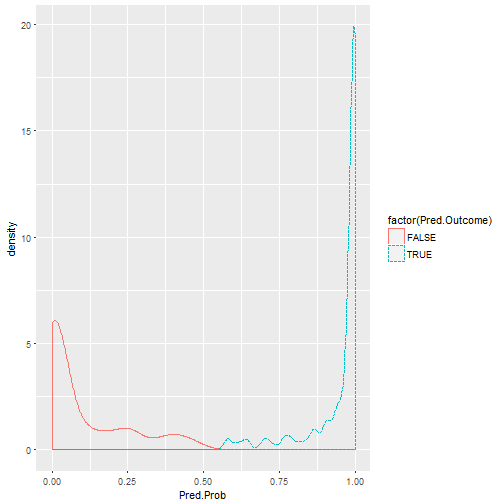
## Sensitivity/Recall (TP) = 0.958 ## Specificity (TN) = 0.932 ## Positive Predictive Value / Precision (All P) = 0.958 ## Negative Predictive Value (All N) = 0.932 ## Overall Accuracy / Hit-rate= 0.948
The accuracy on the training set is 93.6% which is good and close to the original. Sometimes this can go up or down (latter more likely as less data to fit to) and this is a good reason to perform Cross-Validation where we give it different samples, as we will see later.
The accuracy on the validation set (whose original ward level records the model has never been given so it is completely new to it) remains high at 94.8%. This is unusual, being higher than the training set, but is just good luck with the 30% of data it was given to validate.
The model is better at predicting True Positives (Sensitivity / Recall) than True Negatives (Specificity).
Cross-Validation
We would always like to improve the model by giving it as many test cases as possible, yet we don’t want to give them all at once otherwise it will overfit the model – ie become tuned to the exact data rather than underlying correlations, which would make it worse at predicting new data.
So let’s use a cross-validation tool to split the data into K-fold (eg 10) datasets for resampling.
train(Outcome ~ ., data=brexitvote.sub, method='glm', family=binomial, trControl=trainControl(method='cv', number=10))
## Generalized Linear Model ## ## 1029 samples ## 51 predictor ## 2 classes: ‘FALSE’, ‘TRUE’ ## ## No pre-processing ## Resampling: Cross-Validated (10 fold) ## Summary of sample sizes: 927, 926, 927, 926, 927, 927, … ## Resampling results: ## ## Accuracy Kappa ## 0.916 0.824
Note the accuracy corresponds to our earlier model. The Cohen’s Kappa shows the ratio of difference between actual and chance agreement of predictions, with 1 being perfect and 0 showing no better than completely independant agreement. This 83.6% is a good indicator of definitive prediction.
If we provided less predictors, we can see the accuracy and Kappa statistic reduce.
train(Outcome ~ Level.1.qualification.Percent + Level.2.qualification.Percent, data=brexitvote.sub, method='glm', family=binomial, trControl=trainControl(method='cv', number=10))
## Generalized Linear Model ## ## 1029 samples ## 2 predictor ## 2 classes: ‘FALSE’, ‘TRUE’ ## ## No pre-processing ## Resampling: Cross-Validated (10 fold) ## Summary of sample sizes: 926, 927, 925, 925, 926, 927, … ## Resampling results: ## ## Accuracy Kappa ## 0.849 0.677
We can shorten the output whilst including Standard Deviations.
train(Outcome ~ ., data=brexitvote.sub, method='glm', family=binomial, trControl=trainControl(method='cv', number=10))$results
## parameter Accuracy Kappa AccuracySD KappaSD ## 1 none 0.921 0.835 0.0231 0.0481
Conclusion
We have seen that logistic regression can both predict voting behaviour from ward information and demographics, and also pick out deeper demographic voting likelihoods, and use this to build a profile of type of voter.